Really short intro
Given random variable $X$, GAN (Generative Adversarial Nets) aims to learn $P(X)$ via generative methods, specifically, it involves two neural networks playing a minimax game, where one is constantly generating data points that resemble $X ~ P(X)$ to pass it on as a “real” sample, while the other tries to recognize the actual real sample and the generated one, the game goes on until both reach the Nash equalibrium.
The two parts of a GAN are; a generator $G$ and a discriminator $D$. The generator is responsible for sampling from some noise space Z and generate output $G(Z)$, the discriminator tries to learn features that will help distinguish $X$ and $G(Z)$.
During training, $G$ receives penalty from $D$ for doing a bad job at fooling $D$, whilst $D$ receives penalty from not being able to pick $X$ and $G(Z)$ apart. This can be intuitively understood as a competition between the bank and a counterfeiter, the bank loses money if it cannot tell fake money from real ones, the counterfeiter as well would lose his investments into buying equipments if the fake money didn’t pass through.
Objectives of GAN
The objective is as follows
The objective is just binary crossentropy with samples of $x$ set to $1$ and $G(z)$ set to $0$. This is exactly what we want, by maximizing this loss, $D$ would like to classifiy $x$ as 1 and $D(Z)$ as $0$. In contrast, $G$ minimizes the loss in attempts to make $D$ classify $D(z)$ as 1.
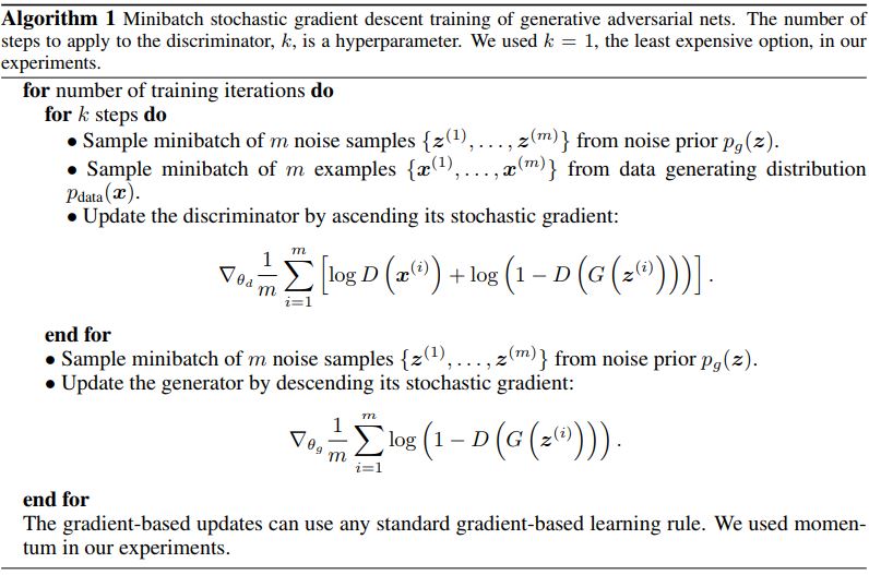
Algorithm
The optimization is carried out iteratively via gradient descent
Analysis of the objective
Optimal $D$
We can find the optimal $D$ by differentiating the objective function.
To maximize this integral, it is sufficient to maximize the integrand, since the integrand is positive inside the interval of integration. The function $f(y) = a \log(y) + b \log(1-y)$ with $y\in [0,1]$, a,b \in $[0, 1]$, attains a maximum in at $\frac{a}{a+b}$. This can be checked by differentiation
So it is indeed a maximum. Plugging the probabilities back we get
In a GAN, we would like $p_g = p_x$, this means $D* = \frac{1}{2}$ as GAN training comes to an end. This make sense as $G(Z)$ looks so real $D$ is no longer able to tell $X$ and $G(Z)$ apart.
Optimal $G$
Now that we know what the optimal $D$ looks like, we can use it to find $G^{*}$.
plugging in $p_g = p_x$ we find that $C(G)= -\log 4$. Intuitively, this should be the minimal value attainable for $C(G)$ from the definition of Nash equilibrium, we just need to prove it’s true. Notice that
By the Jansen inequality, the Jansen-Shannon divergence (JSD) is non-negative and $0$ iff $p_x = p_g$, therefore the minimum attainable value for $C(G)$ is $-\log 4$ and the solution is unique.
A closer look at $C(G)$…
We know now that minimizing $C(G)$ will give us $G^*$, we can do this via gradient descent like usual. But how well does it work?
Early stages of training
We note that $G(Z)$ will not look realistic enough to fool $D$ at the very beginning, this poses danger of $D$ overpowering $G$ so subsequent classification of $G(Z)$ will always be $0$, causing $\frac{\partial D}{\partial G}$ to saturate at $0$ due to sigmodal nature.
Ian Goodfellow [1] suggested to change the optimization objective of $G$ to minimizing $-\mathbb{E}_{p_z} [\log D(G(z))]$. So the gradient now looks like
So even if $\frac{\partial D}{\partial G}$ saturates, the divergent $\frac{1}{D(G(z))}$ will help to provide a non-zero gradient for $G$.
But it’s not that simple, the change in the objective actually causes something known as a mode collapse, which is when $G$ giving up diversity in the generated sample for stability in the objective. We won’t go into that here, interested readers can read this paper [2]
Later stages of training
In general, distributions in high dimensional space resolve into 3 situations, let $p$ and $q$ be distributions over $\chi$ and $\mu$ be a measure.
- $\text{supp}(p) \cap \text{supp}(q) = \emptyset$
- $\text{supp}(p) \cap \text{supp}(q)) \neq \emptyset$ and $\mu(\text{supp}(p) \cap \text{supp}(q)) > 0 $
- $\text{supp}(p) \cap \text{supp}(q) \neq \emptyset$ but $\mu(\text{supp}(p) \cap \text{supp}(q)) = 0 $
1 and 3 are the most worrisome situations for us when calculating JSD, as JSD would evaluate to a constant everywhere, hence the gradient is always zero. As a result, gradient based optimization will certainly fail.
But does this happpen often? The answer is yes, especially when the noise space dimension is much lower than the intrinsic dimension of the dataset and in practice, the noise dimension are around 100 - 300, whereas dimensions of most images are way up in the one-hundred thousands.
As a result, $G$ will always exprience some kind of vanishing graient problem in later stages of training due to a near-optimal $D$, the generated data’s quality thus suffer from the inability of $G$ to improve.
A workaround is adding noise to $X$ in hopes that increasing $\sigma(X)$ will increase $\mu(\text{supp}(p) \cap \text{supp}(q))$. But experimental results have shown including noise will temper with quality of $G(Z)$ [2]
Implementation in Keras
Tricks of training GANs
GANs are notoriously hard to train, due to reasons we gave above. There are tricks to help you train better GANs, see here for a list of collected wisdoms.
Conclusion
GANs can learn the probability density of $X$ implicitly, but it is very hard to train due to the fundamental flaws in the objective functions. In the next blog, we will attempt to solve this once and for all by introducing a better objective that does not possess the shortcomings of the original GAN.
