EM algorithm and mixtures of distributions

As a data scientist in the retail banking sector, it is natural that I do a lot of customer segmentations. Recently I was assigned to investigate on what kind of behavior our investment fund customers exhibit online, I used Gaussian mixture models to see what kind of “in between” After the project was concluded I decided to write a blog about Gaussian mixture as I thought the theory was quite interesting.

Background

Suppose now we are given the following data.

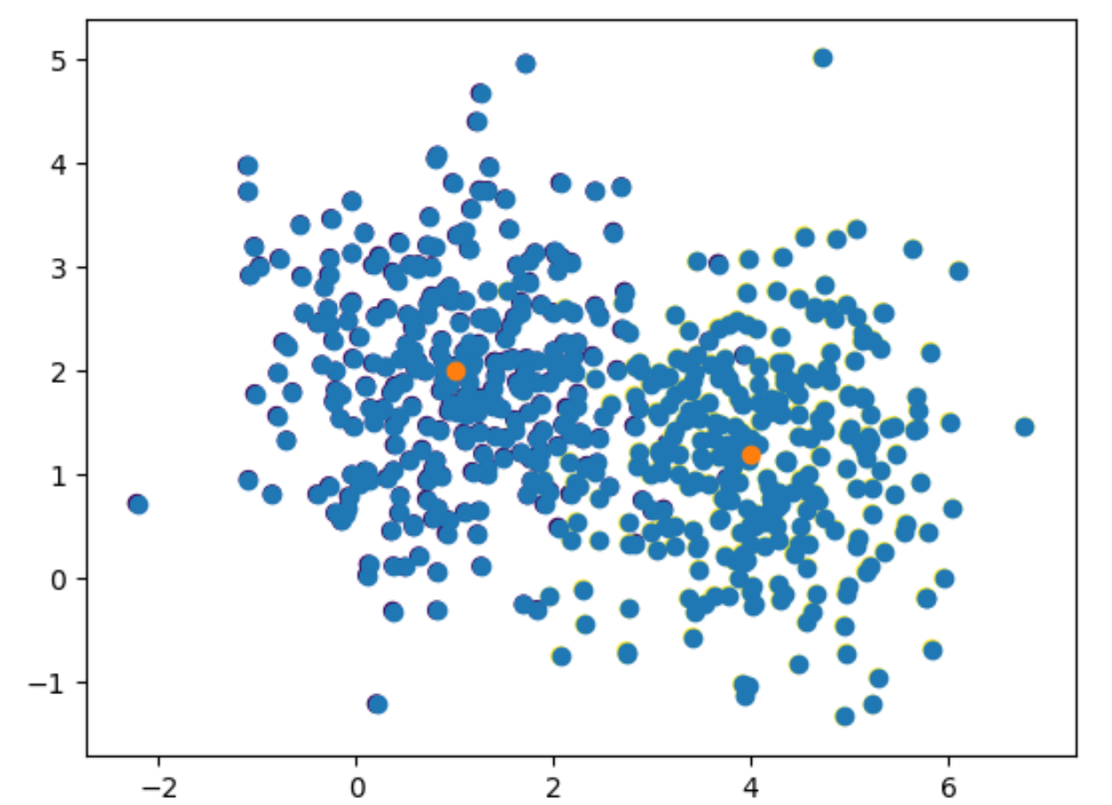
It is quite clear that there are two distinct distributions that generated the data. If this observation is correct, one question of immediate interest is what are the two distributions? Let’s assume that indeed there were only 2 distributions in the generation process. So that for an individual data point, it’s density is

$$\begin{align*} p(x) &= \pi\:p(x\mid \text{first distribution}) + (1-\pi)\:p(x\mid \text{second distribution})\\ &= \pi\:p(x\mid z_k=1) + (1-\pi) P(x\mid z_k=2) \end{align*}$$

where $\pi$ is the weighting of the first distribution, often called the responsbility of first distribution generating $x$, same interpretation is applied to $(1-\pi)$, $z_k$ an indicator of the components.

Note that in the most commonly used cluster algorthm K-Means, the responsibility is binary, meaning that a data point either came from a particular component or it did not, this can affect how we interpret the datapoints that are “in between” geometrically.

To loosen the notation as well as generalize the results we will obtain, let’s assume we have $K$ components instead, so the density is then

$$\begin{align*} p(x) = \sum_{k=1}^K \pi_k\: p(x\mid z_k) \end{align*}$$

Method

We know not how $p(x\mid z_k)$ looks like at this point. But some assumptions can be made to help us estimate the true distribution, for example, let’s assume that $p(x\mid z_k)$ came from some parametric family of distributions so that $p(x\mid z_k) = p(x\mid z_k, \theta)$. Furthermore, let’s further assume that the components are Gaussians so that $p(x\mid z_k, \theta) = \mathcal{N}(x; \mu, \Sigma) $

Once we have that, we can try to use MLE to estimate the parameters that define this distribution. Recall the join distribution of n independent observations is

$$\begin{align*} p(X\mid \theta) &= \prod_{n=1}^N p(x_n\mid \theta) \\ &= \prod_{n=1}^N \sum_{k=1}^K \pi_k\:\mathcal{N}(x_n; \mu_k, \Sigma_k) \end{align*}$$

the log liklihood is then

$$\begin{align} \log p(X; \pi, \mu, \Sigma) = \sum_{n=1}^n \log \sum_{k=1}^K \pi_k\:\mathcal{N}(x_n; \mu_k, \Sigma_k) \end{align}$$

This is quite difficult to maximize, the derivatives are not nice and might cause numerical instability.

Jensen’s inequality

It turns out, we can maximize a lower bound of (1) by invoking the Jensen’s inequality

For any convex function $f:\mathbb{R}\rightarrow \mathbb{R}$, let $S$ be a convex combination $S=\sum_{n=1}^n \alpha_ix_i$, the following is true $$ \begin{align*} f(S) = f(\sum_{n=1}^n \alpha_ix_i) \leq \sum_{n=1}^n \alpha_i f(x_i) \end{align*}$$ if $f$ is concave then the inequality is flipped.

In the language of statistics, this means that $f(\mathbb{E}[X]) \leq \mathbb{E}[f(X)]$.

To use this inequality on our log liklihood, notice that we already have the form required by the theorem, since $\sum \pi_k = 1$. However, using the inequality directly would restrict our model’s flexibility at choosing which component the data was generated from (linear dependence on the $\pi_k$).

So let’s introduce another distribution to take care of the weighting of a cluster for each sample, call it $Q(z_n=k)$

$$\begin{align} \log p(X\mid \pi, \mu, \Sigma) &= \sum_{n=1}^n \log \sum_{k=1}^K \pi_k\:\mathcal{N}(x_n; \mu_k, \Sigma_k)\nonumber \\ &= \sum_{n=1}^n \log \sum_{k=1}^K \pi_k\:\mathcal{N}(x_n; \mu_k, \Sigma_k) \frac{Q(z_n=k)}{Q(z_n=k)} \nonumber\\ &= \sum_{n=1}^n \log \mathbb{E}_{Q(z_n=k)} \:\frac{\pi_k\:\mathcal{N}(x_n; \mu_k, \Sigma_k)}{Q(z_n=k)} \nonumber\\ &\geq \sum_{n=1}^n \mathbb{E}_{Q(z_n=k)} \log\:\frac{\pi_k\:\mathcal{N}(x_n; \mu_k, \Sigma_k)}{Q(z_n=k)} \nonumber\\ &= \sum_{n=1}^n\sum_{k=1}^K Q(z_n=k)\log \frac{\pi_k\:\mathcal{N}(x_n; \mu_k, \Sigma_k)}{Q(z_n=k)} \\ &= l(X, Z, Q) \nonumber \end{align}$$

Tight bound - E step

$Q(Z)$ can be any disitribution in theory, although some choices of $Q$ are better than other ones. In particular, if we can make the above lower bound tight (the log liklihood is exactly equal to the lower bound) by choosing the right $Q$, then we can get some nice properties out of it.

To find such $Q$, we take at the difference between $\log p(X\mid \theta)$ and $l$. For a single data point x, we have

$$\begin{align*} \log p(x\mid \theta) - l(x, Z, Q) &= \log p(x\mid \theta) - \sum_{k=1}^K Q(z=k)\log \frac{\pi_{k}\:\mathcal{N}(x; \mu_k, \Sigma_k)}{Q(z=k)}\\ \\ &= \log p(x\mid \theta) \sum_{k=1}^K Q(z=k) - \sum_{k=1}^K Q(z=k)\log \frac{\pi_{k}\:\mathcal{N}(x; \mu_k, \Sigma_k)}{Q(z=k)}\\ \\ &= \sum_{k=1}^K Q(z=k)\left(\log p(x\mid \theta) - \log \frac{\pi_{k}\:\mathcal{N}(x; \mu_k, \Sigma_k)}{Q(z=k)} \right)\\ \\ &= \sum_{k=1}^K Q(z=k)\log \frac{p(x\mid \theta)\:Q(z=k)}{\pi_k\:\mathcal{N}(x; \mu_k, \Sigma_k)}\\ \\ &= \sum_{k=1}^K Q(z=k)\log \frac{Q(z=k)\sum_{i=1}^K \pi_i\:\mathcal{N}(x; \mu_i, \Sigma_i)}{\pi_k\:\mathcal{N}(x; \mu_k, \Sigma_k)}\\ \\ &= \sum_{k=1}^K Q(z=k)\log \frac{Q(z=k)}{\pi_k\:\mathcal{N}(x; \mu_k, \Sigma_k) / \sum_{i=1}^K \pi_i\:\mathcal{N}(x; \mu_i, \Sigma_i)}\\ \\ &= \text{KL}\left(Q(z=k) \Big|\Big| \frac{\pi_k\:\mathcal{N}(x; \mu_k, \Sigma_k)}{\sum_{i=1}^K \pi_i\:\mathcal{N}(x; \mu_i, \Sigma_i)}\right) \end{align*}$$

Since the KL divergence is non-negative, it is sufficient to set

$$\begin{align} Q(z=k) = \frac{\pi_k\:\mathcal{N}(x; \mu_k, \Sigma_k)}{\sum\limits_{i=1}^K \pi_i\:\mathcal{N}(x; \mu_i, \Sigma_i)} \end{align}$$

to attend a tight bound. In our optimization procedure, this is called the E step or Expectation step.

The $Q$ we have acquired will help us prove the convergence of our iterative algorithm later.

Maximization - M step

It’s time we carry out the maximization, for this particular problem of fiitting mixture of Gaussians, some matrix calculus identities will be useful, refer to this SO page for more details.

Recall the formula for a multivariate Gaussian distribution

$$\begin{align*} \mathcal{N}(x; \mu, \Sigma) &= \frac{1}{\sqrt{(2\pi)^M\det(\Sigma)}}\exp(-\frac{1}{2}(x-\mu)^T\Sigma^{-1}(x-\mu))\\ \log \mathcal{N}(x; \mu, \Sigma) &= -\frac{1}{2} \left( \log(\det(\Sigma)) + (x-\mu)^T\Sigma^{-1}(x-\mu) + M\log 2\pi\right) \end{align*}$$

Refering back to the optimization objective (2), our $l$ now becomes

$$\begin{align*} \small{ \sum_{n=1}^N\sum_{k=1}^K Q(z_n=k)( \log\pi_k -\frac{1}{2} ( \log\det(\Sigma_k^{-1}) - (x-\mu_k)^T\Sigma_k^{-1}(x-\mu_k) + M\log 2\pi)) - Q(z_n=k)\log Q(z_n=k)} \end{align*}$$

The respective optima are

$$\begin{align} \frac{\partial l}{\partial \mu_k} &= \sum_{n=1}^N 2Q(z_n=k)\Sigma_k^{-1}(x_n-\mu_k) = 0\nonumber\\ \Rightarrow \mu_k &= \frac{\sum\limits_{n=1}^N Q(z_n=k)x_n}{\sum\limits_{n=1}^N Q(z_n=k)}\\ \frac{\partial l}{\partial \Sigma_k} &= \frac{1}{2}(\sum_{n=1}^N Q(z_n=k)(\frac{\partial}{\partial \Sigma_k} \log\det\Sigma_k - \frac{\partial}{\partial \Sigma_k} (x-\mu_k)^T\Sigma_k^{-1}(x-\mu_k))\nonumber\\ 0 &= \frac{1}{2} \sum_{n=1}^N Q(z_n=k) (\Sigma_k^{-T} - \Sigma_k^{-T}(x-\mu_k)(x-\mu_k)^T\Sigma_k^{-T} )\nonumber\\ \Rightarrow \sum_{n=1}^N Q(z_n=k) &= \sum_{n=1}^N Q(z_n=k)(x-\mu_k)(x-\mu_k)^T\Sigma_k^{-T}\nonumber \\ \Rightarrow \Sigma_k &= \frac{\sum\limits_{n=1}^N Q(z_n=k)(x-\mu_k)(x-\mu_k)^T}{\sum_\limits{n=1}^N Q(z_n=k)} \end{align}$$

For the $pi_k$, we need to apply some constraints for them to be proper distributions, they are $\sum_k \pi_k = 1$ and $\pi_k\geq 0 :\forall k=1\cdots K$. Using the KKT conditions, we solve the following system of equations

$$\begin{align*} \nabla\mathcal{L} = \nabla(-\sum_{n=1}^N\sum_{k=1}^K Q(z_n=k)\log\pi_k +\sum_{k=1}^K\mu_k\pi_k - \lambda (\sum_{k=1}^K\pi_k - 1)) = 0\\ \sum_{k=1}^K\pi_k - 1 = 0\\ \pi_k\geq 0 \:\forall k=1\cdots K\\ \mu_k\geq 0 \:\forall k=1\cdots K\\ \mu_k\pi_k^{\ast} = 0 \end{align*}$$

Now to actually solve the constrained optimization problem $\begin{align} \nabla\mathcal{L} &= -\sum_{n=1}^N \frac{Q(z_n=k)}{\pi_k} + \mu_k - \lambda = 0 \nonumber \\ &\Rightarrow -\sum_{n=1}^N Q(z_n=k) + \mu_k\pi_k - \lambda \pi_k = 0 \nonumber\\ &\Rightarrow -\sum_{n=1}^N\sum_{k=1}^K Q(z_n=k) - \sum_{k=1}^K\lambda \pi_k = 0 \nonumber\\ &\Rightarrow -N - \lambda = 0 \nonumber\\ &\Rightarrow \lambda = N \nonumber \\ &\Rightarrow \pi_k = \frac{1}{N} \sum\limits_{n=1}^N Q(z_k=n) \end{align}$

Summary of EM algorithm

Implementation of GMM EM in Python

In this implementation, I used some scipy functions for convenience, they can be swapped out to make it purely numpy based.

Experimentation

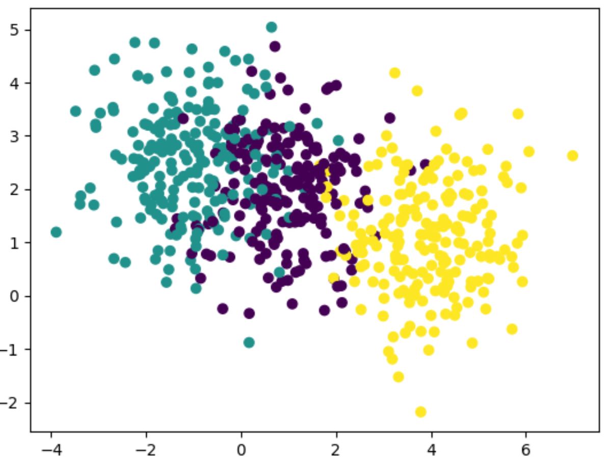
I have generated a dataset that came from three distributions, these are generated with labels so we can assess the quality of our clustering directly.

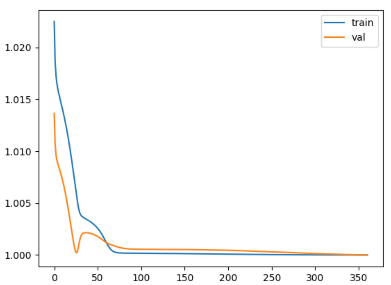
I ran GMM for 60 iteration and return a classfication report from sklearn. The number of iteration can be determined by performing validation on lower bound provided in (2), or perform early stopping.

Label	Precision	Recall	f1-score	Support
0	0.90	0.50	0.67	51
1	0.76	0.94	0.84	51
2	0.84	0.91	1.00	48