 This is one problem that practioners in data science often face, it is caused by difference between the distributions of training and testing set.
Lack of "robustness" in the neural network is what's causing the problem, a small change in the input causes big change in the output.
On top of that, autoencoders do not introduce variety, the output, in theory, should always be a member of the training set, since this is what it is trained to do. If this is the case, then we have done no better than to copy the dataset twice or thrice. Can we address that problem too?
### Denoising autoencoder
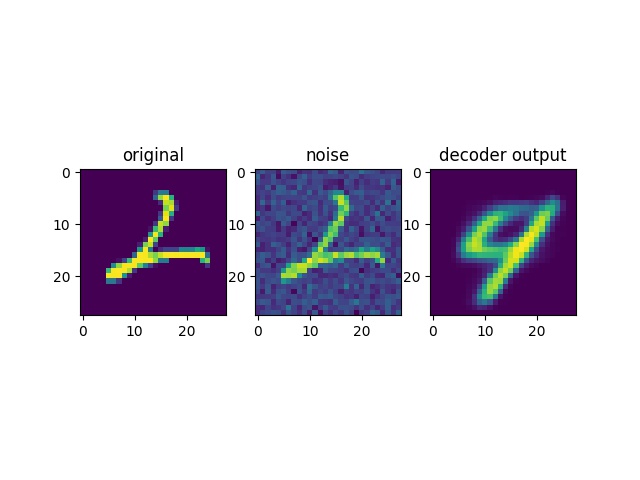
Denoising autoencoder tries to solve problem 1 (lack of robustness) by directly corrupting the training sample, and then reconstructing the uncorrupted sample. This process forces the encoder to discover more robust features during training, thus allowing the encoder to have better "locallity", ie
So given a sample $X$, define a transformation as folllows
$$ g(X) = X + \epsilon $$
we introduced a noise parameter $\epsilon \sim P$, where $\epsilon$ is a random variable with distribution $P$. This is the easiest way one can use to corrupt the dataset,in practice one chooses $\epsilon \sim \mathcal{N}(\mu, \sigma^2)$
So the whole problem can be summed up as, finding $\phi: \Omega\rightarrow \mathcal{F}$, $\psi: \mathcal{F}\rightarrow \Omega$
$$ \phi, \psi = \mathop{\arg\ \min}\limits_{\phi, \psi}' ||X - (\psi \circ \phi \circ g) X||^2 $$
Using the mnist dataset again as an example
{% gist c3292a782d87cce26daaed659108bfb5 %}

### Contractive autoencoder
Contractive autoencoder tries to solve the same problem by directly limiting the change of the latent representation with respect to the input. By increasing the flatness around the training examples in the latent space, we can limit the rate of change of the representation with respect to the input, and that's what we meant by robustness. In terms of math, this is to minimize the derivative matrix around the training example, one way to do so is regularizing $\partial \phi(x)/ \partial (x)$. The objective now becomes
$$ \phi, \psi = \mathop{\arg\ \min}\limits_{\phi, \psi} ( ||X - (\psi \circ \phi) X||^2 + \lambda \:\left|\left|\frac{\partial \phi_j(X_i)}{\partial X_i}\right|\right|^2)$$
$\lambda$ is a hyperparameter that determines the regularization strength.
### Variational autoencoder
This is one problem that practioners in data science often face, it is caused by difference between the distributions of training and testing set.
Lack of "robustness" in the neural network is what's causing the problem, a small change in the input causes big change in the output.
On top of that, autoencoders do not introduce variety, the output, in theory, should always be a member of the training set, since this is what it is trained to do. If this is the case, then we have done no better than to copy the dataset twice or thrice. Can we address that problem too?
### Denoising autoencoder
Denoising autoencoder tries to solve problem 1 (lack of robustness) by directly corrupting the training sample, and then reconstructing the uncorrupted sample. This process forces the encoder to discover more robust features during training, thus allowing the encoder to have better "locallity", ie
So given a sample $X$, define a transformation as folllows
$$ g(X) = X + \epsilon $$
we introduced a noise parameter $\epsilon \sim P$, where $\epsilon$ is a random variable with distribution $P$. This is the easiest way one can use to corrupt the dataset,in practice one chooses $\epsilon \sim \mathcal{N}(\mu, \sigma^2)$
So the whole problem can be summed up as, finding $\phi: \Omega\rightarrow \mathcal{F}$, $\psi: \mathcal{F}\rightarrow \Omega$
$$ \phi, \psi = \mathop{\arg\ \min}\limits_{\phi, \psi}' ||X - (\psi \circ \phi \circ g) X||^2 $$
Using the mnist dataset again as an example
{% gist c3292a782d87cce26daaed659108bfb5 %}

### Contractive autoencoder
Contractive autoencoder tries to solve the same problem by directly limiting the change of the latent representation with respect to the input. By increasing the flatness around the training examples in the latent space, we can limit the rate of change of the representation with respect to the input, and that's what we meant by robustness. In terms of math, this is to minimize the derivative matrix around the training example, one way to do so is regularizing $\partial \phi(x)/ \partial (x)$. The objective now becomes
$$ \phi, \psi = \mathop{\arg\ \min}\limits_{\phi, \psi} ( ||X - (\psi \circ \phi) X||^2 + \lambda \:\left|\left|\frac{\partial \phi_j(X_i)}{\partial X_i}\right|\right|^2)$$
$\lambda$ is a hyperparameter that determines the regularization strength.
### Variational autoencoder
Autoencoder (part 2)
### What's new?
Continuing the journey through generative models, is part 2 of autoencoder. In the last post, we talked about what an autoencoder is and what are some of its goods and bads. If you don't remember/ don't know what an autoencoder is, I ***highly*** suggest you to read my previous post first.
We had an example of why autoencoders are not perfect, namely, it is very sensitive to the input object. If the input is slightly distorted, the resulting reconstruction could be dramatically different from the original.
This is one problem that practioners in data science often face, it is caused by difference between the distributions of training and testing set.
Lack of "robustness" in the neural network is what's causing the problem, a small change in the input causes big change in the output.
On top of that, autoencoders do not introduce variety, the output, in theory, should always be a member of the training set, since this is what it is trained to do. If this is the case, then we have done no better than to copy the dataset twice or thrice. Can we address that problem too?
### Denoising autoencoder
Denoising autoencoder tries to solve problem 1 (lack of robustness) by directly corrupting the training sample, and then reconstructing the uncorrupted sample. This process forces the encoder to discover more robust features during training, thus allowing the encoder to have better "locallity", ie
So given a sample $X$, define a transformation as folllows
$$ g(X) = X + \epsilon $$
we introduced a noise parameter $\epsilon \sim P$, where $\epsilon$ is a random variable with distribution $P$. This is the easiest way one can use to corrupt the dataset,in practice one chooses $\epsilon \sim \mathcal{N}(\mu, \sigma^2)$
So the whole problem can be summed up as, finding $\phi: \Omega\rightarrow \mathcal{F}$, $\psi: \mathcal{F}\rightarrow \Omega$
$$ \phi, \psi = \mathop{\arg\ \min}\limits_{\phi, \psi}' ||X - (\psi \circ \phi \circ g) X||^2 $$
Using the mnist dataset again as an example
{% gist c3292a782d87cce26daaed659108bfb5 %}

### Contractive autoencoder
Contractive autoencoder tries to solve the same problem by directly limiting the change of the latent representation with respect to the input. By increasing the flatness around the training examples in the latent space, we can limit the rate of change of the representation with respect to the input, and that's what we meant by robustness. In terms of math, this is to minimize the derivative matrix around the training example, one way to do so is regularizing $\partial \phi(x)/ \partial (x)$. The objective now becomes
$$ \phi, \psi = \mathop{\arg\ \min}\limits_{\phi, \psi} ( ||X - (\psi \circ \phi) X||^2 + \lambda \:\left|\left|\frac{\partial \phi_j(X_i)}{\partial X_i}\right|\right|^2)$$
$\lambda$ is a hyperparameter that determines the regularization strength.
### Variational autoencoder